The purpose of this post is to serve partly as a review of Terry Rudolph’s book Q is for quantum and partly as a record of my thoughts after a few months of reading about quantum computation. The first part of Ruldolph’s book may be downloaded for free from his website.
Part 1: Q-computing
The PETE box and the Stern–Gerlach experiment
Q is for quantum begins with a version of the Stern–Gerlach experiment. We are asked to imagine that black and white balls are sent through a box called ‘PETE’. (The afterword makes clear the name ‘PETE’ comes from Rudolph’s collaborator Pete Shadbolt.) After a black ball goes through a PETE box, it is observed to be equally likely to be black and white. The same holds for white balls.
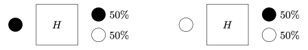
No physical experiment can distinguish the black balls that come out from the black balls that come in, or a white ball that comes out from a white ball from the supply of fresh balls. For example, if the white balls that come out are discarded, and the black balls that come out are passed through a second PETE box, then again the output ball is equally likely to be black and white.

The surprise comes when PETE boxes are connected so that a white ball put into the first one passes immediately into the second. Now the output is always white.
Naturally we are suspicious that, despite our earlier failure to distinguish balls output from PETE boxes from fresh balls, the first PETE box has somehow ‘tagged’ the input ball, so that when it goes into the second box, the second PETE box knows to output a white ball. When we test this suspicion by observing the output of the first PETE box, we find (as expected) that the output of the first box is 50/50, but so is the output of the second. Somehow observation has changed the outcome of the experiment.
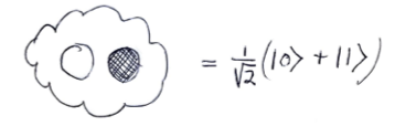
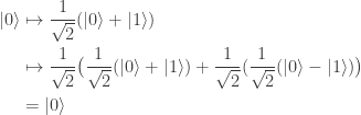
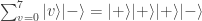
This should already seem a little surprising. But if we accept that observed balls coming out of PETE are experimentally indistinguishable from fresh balls then, Rudolph argues, we have to make a more radical change to our thinking: there is no way to interpret the state of an unobserved ball midway between two PETE boxes as either black or white. As Rudolph says, ‘We are forced to conclude that the logical notion of “or” has failed us’. This quickly leads Rudolph to introduce an informal idea of superposition and his central concept of a misty state. For example, the state  shown above is drawn as the diagram below.
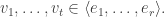
Rudolph then makes the bold step of supposing that when a black ball, represented by  is put through PETE, the output is
  ; of course this is drawn in his book as another misty state, this time with a minus sign attached to the black ball. Does this minus sign contradict the experimental indistinguishability of output balls? I’ll quote Rudolph’s explanation of this point since it is so clear, even though (alas) it contains the one typo I found in the entire book (page 19):
But it isn’t a “physically different” type of black ball; if we looked at the ball at this stage we would just see it as randomly either white or black. No matter what we do, we won’t be able to see anything to tell us that when it we see it black [sic] it is actually “negative-black”.
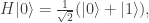
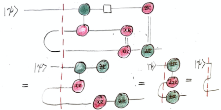
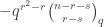
In the mathematical formalism, this is the unobservability of a global phase (a consequence of the Born rule for measurement). Thus in a sense the PETE box does tag the black balls, but not in a way we can observe. The behaviour of a white ball sent into two PETE boxes in immediate succession is easily explained using superposition. The mathematical calculation
is not significantly shorter than Rudolph’s equivalent demonstration using misty diagrams on page 20. His book shows impressive economy by explaining many of the key ideas in quantum theory and computation using just these misty diagrams to compute with the PETE box and certain carefully chosen initial states.
Indeed, Rudolph has already shown one fundamental idea: if we accept that the misty state drawn above is a complete description (much more on this later) of a ball leaving a PETE box, then we have to give up on determinism. Instead the universe is fundamentally random. This was difficult for the early architects of quantum theory to accept, since it contradicts the idea that all physical properties have a definite value. Things are perhaps easier for us now: on the quantum side we are used to the uncertainty principle, and I’d argue that the complexity of modern life, and our relentless exposure to probabilistic and statistical reasoning, makes it easier for us to accept that randomness might be ‘hard-wired’ into the laws of physics. We return to these subtle points after the discussion of Part 2 of Rudolph’s book, where we follow Bell’s argument in refuting the ‘local hidden variable’ theory that, even though we cannot observe it for ourselves, PETE boxes are deterministic, and emit balls tagged in such a way that the laws of physics conspire to agree with the predictions from the misty state theory.
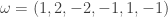
Translating from misty diagrams to the usual bra/ket formalism is of course routine. As one might hope, this infusion of mathematics has some advantages. For instance, if we accept the Born rule that measuring  in the orthogonal basis
  ,
,  gives with probability
  and
and  with probability
  , then conservation of probability requires that this state evolves by unitary transformations in
  . Rudolph’s ‘bold’ step is now forced: once we have
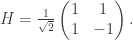
unitary dynamics requires that, up to a phase,
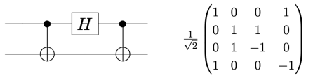
Thus, as my notation in the diagrams above suggests, the PETE box is the Hadamard gate
The Stern–Gerlach experiment shows further quantum effects which are not captured by Rudolph’s thought experiment. In the original experiment, silver atoms were sent through a magnetic field, strongest at the top of the apparatus and weakest at the bottom. The atomic number of silver is

and correspondingly there is a single electron in the 4f subshell. The behaviour of the atom in the magnetic field in the experiment is determined by the spin of this electron. After passing through the magnetic field, two beams of atoms are observed: one deflected upwards and one deflected downwards. The amount of deflection is constant, showing the quantisation of the spin of this single electron.
Rudolph’s thought experiment corresponds to an extended version of this experiment, in which two different fields are used. Interpreting  as `spin up’, the diagram below shows atoms, prepared in the spin-up state by a vertical field, being deflected first by a horizontal magnetic field and then a second horizontal field in the combiner (this field has the reverse gradient to the first horizontal field), and finally a third vertical magnetic field identical to the first one.
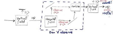
If the atoms are observed in the middle part of the apparatus (shown by a blue box above), or if one of the ‘mirrors’ indicated by diagonal lines is replaced with a barrier, then the output is 50%/50% (red text above). This is interpreted on the Wikipedia page as
… the measurement of the angular momentum on the  direction destroys the previous determination of the angular momentum in the
  direction.
But if the atoms are not observed in the middle, then the output from the final vertical field is 100% spin-up, as for the output from the first vertical field. This holds even if the blue part of the apparatus, in which the horizontal field polarises electrons horizontally into two different beams, sends the atoms on a round trip of thousands of kilometres. As long as, they meet up at the combiner (without observation at any stage), the same interference occurs, and the output from the final vertical field is always spin-up. Since Rudolph’s thought experiment has no analogue of horizontal polarisation, this feature is not captured. But Rudolph has already made a convincing (and entirely honest) case that quantum phenomena cannot be understood by classical physics or conventional probability.
For a detailed account of the physics of the Stern–Gerlach experiment I found these notes useful. See Figure 6.9 for the experiment shown schematically above. Also I highly recommend this MIT lecture by Allan Adams for an entertaining and instructive treatment of the Stern–Gerlach experiment that has some features in common with Rudolph’s presentation, for instance, the use of colour to replace the spin-up and spin-down states , ; he also brings in `hardness’ to replace horizontal polarisation and the states  ,
,  seen in the blue part of the diagram above.
Bank vaults and the Deutsch–Josaz algorithm
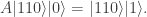
Part I ends with an illustration of quantum computing. We are asked to imagine that thieves have broken into a bank vault, in which each room is stocked with eight golden bars, numbered from  up to
up to  . In some rooms, all bars are fake (‘all that glistens is not gold’); in other rooms, there are four fake bars and four real bars. Happily each room has an ‘Archimedes’ machine, that given as input the ball sequence encoding the bar number in binary and one extra ball, flips the colour of the extra ball if and only if the bar is genuine. For example since
  is
is  in binary, the input balls encoding are black, black, white. We could use either colour for the extra ball. If we use white, then, supposing that bar is genuine, the output is
Moving the result from the  -basis
  to the
  -basis,
 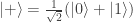 ,
,  we may rewrite this as
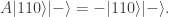
Less happily for them, the thieves only have time to use the Archimedes machine once. The ingenious solution is to apply Archimedes to a superposition of the numbers of all  bars, created by three white balls put into three PETE boxes in parallel, with the extra ball in the state
  , created by putting a black ball into a PETE box. The input is therefore
  and the output is

where  if bar
  is fake, and
  if bar is genuine. If all bars are fake then the output is
in agreement with the input. In this case, measuring in the basis must give . Suppose instead that the vault has an even split. Since

measuring in the basis cannot give  . Therefore one use of Archimedes suffices to distinguish the two classes of room.
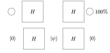
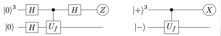
My account here differs from Rudolph’s only in measuring in the -basis rather than applying a further three PETE boxes to move the first three balls back to the -basis, where they can be measured (in the only way possible in his book) by inspecting their colour. This change replaces an operation with a computational flavour (applying three  gates in parallel) with mere linear algebra (just express the output in the -basis). Similary I prefer to think of the input as the product state
  in the -basis rather than as the result of four gates applied to the product state
  in the -basis. Of course this reflects my perspective that quantum computation is hard but (after 25 years of it) linear algebra is easy. The change of perspective is shown in the two circuit diagrams below.
Rudolph can’t employ these dodges and instead gives a `proof by example’ for the even split case, using an alphabetic notation for the final misty state in the -basis:

with  entries. The reader is invited to check that the coefficient of WWW is zero. With the exception of the final discussion of ‘ontic states’, this is probably the hardest part of the book, as clearly the author was aware, writing ‘Even if you raced through all that (as I would do on a first reading) and didn’t really follow it, that’s OK.’ Besides the jump in difficulty, a possible weakness of this section is the contrived nature of the problem. This however reflects the history of the subject: the Deutsch–Josaz algorithm was one of the earliest instances of quantum speed-up over classical algorithms. Rudolph illustrates this speed-up by considering a vault with 65536 gold bars.
I think it is a little too tempting to conclude from Rudolph’s exposition that quantum computers are, at least for some tasks, strictly superior to classical computers. This however is unproved: the subtle point is that in any algorithmic specification of the problem, the Boolean function  either has to be treated as an oracle, in which case the Deutsch–Josaz algorithm only proves the weaker result that relative to an oracle quantum computers are superior to classical computers, or given as part of the input, in which case it is no longer clear that there is no better classical algorithm than evaluating
  at
at  of the inputs.
Still, this section is a nice illustration that quantum computers derive their power from interference, and not just (as Rudolph very clearly explains on page 50) from the superposition of exponentially many states. The reversible nature of quantum computing also emerges quite naturally from the white/black ball model and the use of the fourth ball in the input to Archimedes, but Rudolph chooses not to comment on this.
Part 2: Q-entanglement
This part, the highlight of the book for me, has an exceptionally clearly presented and improved version of the EPR-paradox. I’ll begin by giving my version of the original, separate from the more philosophical concerns of Einstein, Podolsky and Rosen, which I discuss in the final part.
The EPR-paradox as it seems now
Let  be
be  -dimensional Hilbert space modelling a single qubit, with -basis
  ,
,  . Alice and Bob have shared the Bell state
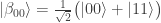
so that Alice has control of the first qubit and Bob the second. If all Alice and Bob can do is measure their qubit in the -basis then  behaves exactly like a shared (but unknown) classical bit: for each
  when Alice measures
  , she can be certain Bob will also measure , and vice-versa.
To motivate the next step we observe that  is not, as might seem from the formula above, in any way tied to the -basis. For instance, it is easy to check that

and in fact this formula holds replacing  with any orthonormal basis of . It follows that Alice and Bob can measure in any pre-agreed basis
  of , and obtain the same classical bit. This suggests they might also try measuring in different bases. Let Alice’s basis (for the first qubit) be

and let Bob’s basis (for the second qubit) be

Thus Alice’s basis  is obtained by rotating the -basis by
  , and Bob’s basis
  by rotating the -basis by
  . It follows, by considering the inverse rotation, that
  and
and  . There are of course similar expressions for the -basis elements in terms of Bob’s basis, obtained by replacing with . Using these we obtain
For instance if  then
then 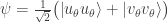 , so Alice and Bob either both measure
  or both measure , as we claimed above. In particular, as already remarked, if Alice and Bob agree to measure in the -basis, so
  then when Alice measures
  she can be sure Bob will also measure
  . If instead
  then the other two summands vanish and Alice measures
  if and only if Bob measures
  . If
. If  then there is no correlation between Alice’s measurement and Bob’s measurement. In particular, if Alice and Bob agree that Alice will measure in the -basis and Bob will measure in the -basis then Bob is equally likely to measure as , irrespective of Alice’s measurement.
In general, by the Born rule, if  then the probability that Alice and Bob obtain the same result (i.e. either for Alice and
  for Bob or
  for Alice and for Bob) is
  . All this leaves no doubt that Alice’s measurement affects Bob’s. This is the spooky ‘action at a distance’, or non-locality, that so bothered Einstein. We defer further discussion to Part 3, and instead present the main result from Bell’s 1964 paper, written 29 years after Einstein, Podolsky and Rosen.
Bell’s game
We suppose that Alice and Bob are, as is usual in the tortured circumstances of thought experiments in quantum mechanics, held in isolated Faraday cages 20 light years apart. They are made to play the following game. The Gamesmaster chooses two classical bits and tells Alice  and Bob
  . Alice and Bob must each submit further classical bits
  and
and  . They win if
  . That is, if
  then Alice and Bob win if and only if they guess the same, and if
  then Alice and Bob win if and only if they guess differently.
Using a single shared (but unknown) classical bit, or equivalently, by only measuring the Bell state in the same pre-agreed basis, Alice and Bob can win with probability  . One simple strategy is to ignore and entirely and simply submit their shared classical bit. In this case
  and our heroes win if and only if , which holds with probability . In another strategy Alice submits and Bob submits ; since
  except when
  and
and  , again the winning probability is . (This strategy makes no use of their shared bit.) It is not hard to convince oneself that, provided the Gamesmaster plays optimally, for instance by choosing and independently and uniformly at random, no better strategies are available. This holds even if Alice and Bob are allowed to use their own (independent, classical) sources of randomness before deciding what to submit.
By measuring in different bases, Alice and Bob can do strictly better. It is clear that if Alice is told  , she wants to choose a basis that must be close to Bob’s, while if Alice is told , then she wants a basis close to Bob’s when , and a basis rotated by nearly a right angle when
  . Bob is of course in the same position. Thinking along these lines one can show that a good choice of bases for the measurements (each basis depending only on the classical bit each of them is told) is as follows:
- For Alice: if take
 , if take
  ;
;
- For Bob: if take
 , if take
  .
.
These bases are shown in the diagram below.
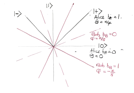
Note that Alice’s basis is the -basis  when and the -basis when . This collection of all four bases is in fact the unique optimal configuration, up to rotations and reflections.
Checking the four cases for  shows that if then the bases chosen by Alice and Bob differ by an angle of
  . Therefore Alice and Bob measure in nearby bases and submit identical bits with probability
  , winning with probability
  . If then the bases chosen by Alice and Bob differ by an angle of
  . The probability that Alice and Bob submit identical bits is now
  . Since their aim now is to submit different bits, they win again with probability .
To give an explicit example, suppose that , so Alice measures in the -basis, and so Bob measures in the basis rotated by  . The relevant form for
  is
is
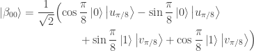
and so, as just claimed, the probability that either Alice measures and Bob measures  or Alice measures
  and Bob measures
  is
is 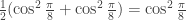 .
.
The Gamesmaster can arrange that Alice and Bob are told and at the same time, and must then reply within a few seconds. (To take into account special relativity, we put Aice at the origin and Bob in a position space-like separated from Alice so that in any reference frame light takes more than the allowed number of seconds to travel from Alice to Bob.) This rules out even one way communication between Alice and Bob, unless they can employ a particle travelling faster than light. By applying a Lorentz transform one can convert any FTL-communication into a violation of causality. It is inconceivable that Alice’s qubit somehow transmits the result of Alice’s measurement to Bob’s qubit. But still, by choosing their bases carefully, Alice and Bob are able to influence the strength of the correlation (or anti-correlation) between their two measurements to the extent that they can play the game strictly better than classical physics allows. All this follows just from the Born rule for measurement and the simple rule proved above for how the Bell state transforms under two different rotations.
Rudolph’s improved version
To make a convincing demonstration of the improvement from the classical winning probability to , Alice and Bob would of course have to play the game multiple times, and accept that they will lose with probability about 15%. For instance, after 100 trials with 85 successes, one would reject the null-hypothesis that Alice and Bob are using a classical strategy with confidence specified by the  -value
  .
.
In Part 2, Rudolph offers an improved version of the EPR-paradox, using a game with three outcomes (win, draw, lose) in which, by using a suitable entangled -qubit state, Alice and Bob can sometimes win and guarantee never to lose. Rudolph’s ingenious construction means that only measurements in the – and -basis are required, so (making the same shift from measurement-in-arbitrary-basis to computation-by-unitary-operator-and--basis measurement remarked on earlier) Alice and Bob can work the magic using only black and white balls and the PETE box. Rudolph sets things up very carefully, in the entertaining context of Randi’s well known million dollar price for an experimentally testable demonstration of telepathy (or indeed, any psychic phenomenon). In particular, my claim above that no classical strategy can beat in the EPR-game becomes the claim that any classical strategy in Rudolph’s game that has a non-zero winning probability also has a non-zero losing probability: this is convincingly shown in the narrative.
Part 2 ends with a discussion of just what is paradoxical about the games. Rudolph argues that a causal explanation of the nonlocal correlation in misty states is inconsistent with our understanding that causes precede effects, and that information cannot be transmitted faster than light. He remarks ‘physicists seriously consider other disturbing options’, for instance the super-deterministic theory where the bits and and Alice and Bob’s strategy (and even, whether or not Alice and Bob will follow their strategy as instructed) are already ‘known’ to the entangled qubits. Another possibility is that Rudolph’s ‘misty state’, modelling the two entangled qubits, is in fact ‘some kind of real physical object like a radio wave or a bowl of soup, and when we separate the psychics the mist is stretched between them’. (Rudolph is very clear that until this point, the misty states have been a mathematical abstraction, just as my calculations with unitary matrices above.)
Part 3: Q-reality
It is both a strength and weakness of Q is for quantum that at this point it is very tempting to throw up one’s hands and say ‘okay, I’m convinced misty states are the best approximation to reality there is, non-locality and paradoxical behaviour accepted’. I think this is particularly tempting for mathematicians — surely a theory of such beauty and explanatory power has to be ‘right’? As a partial corrective to this, let me break from following Rudolph’s book, and instead consider the EPR-paradox in its historical context. We follow this with a discussion of quantum teleportation, before rejoining Rudolph’s final chapter.
Rocky states and the EPR-paradox as presented by the authors
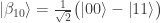
At the end of Part 2, Rudolph introduces the idea of a ‘rocky state’, namely a classical probability distribution on physical states. He shows that the entanglement in the Bell state  cannot be explained in this way: in mathematical language, a classical probability distribution that gives some probability to the observations
  and
and  for both Alice and Bob must give a non-zero probability to
  , but this has coefficient zero in
  . This supports his conclusion that quantum theory (rather than classical probability) is required to explain the EPR-paradox.
Whatever the status of misty states, rocky states are certainly epistemic: on page 103 early in Part 3, Rudolph writes `the rocky states are unquestionably representing our knowledge’. For example, if I borrow a coin from Malcolm and flip it on a table, and see roughly how far it is from the edge, my rocky state might be as shown left below. Malcolm however knows his coin is double-headed, so his rocky state is as shown on the right.
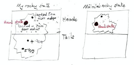
As Rudolph writes (page 104),
the very fact that two different rocky states can correspond to the same real state indicates that the rocky states themselves are not a physical property of the coin.
So far, so clear, I hope. It is therefore striking that a very similar argument led Einstein, Podolsky and Rosen to conclude that misty states could not be in bijection with real states. To understand this, I think one must first appreciate that the authors took at one of the starting points in their paper that particles had real physical properties that were revealed by observation. Some version of this view, ‘scientific realism’, is implicit in the scientific method, and helps to explain its power. (We used it earlier, when we deduced from the experimental indistinguishability of balls output by the PETE box from fresh balls that there was a fundamental randomness in the laws of physics.) As a working definition, let me define naive realism to mean that an output ball from a PETE box is definitely either black or white — we just don’t know what it is until observation. Equivalently, the -basis state  is a convenient mathematical representation for a real state that, on observation, turns out to be either or
  . Thus, in naive realism, quantum states are incomplete descriptions of real states, and the real states have deterministic non-random behaviour.
Suppose as in the exposition of the EPR-paradox in Part 2, that Alice and Bob share the entangled Bell state , but now separated by (let us say) 10 light seconds, and that Bob refuses to measure until he hears that Alice has done so. Suppose that Bob always measures in the -basis. We saw that if Alice also measures in the -basis then Alice and Bob are guaranteed to get the same -basis measurement, while if Alice measures in the -basis, Bob is equally likely to get as , whatever Alice measures. This agrees with the predictions of the extended version of the Born rule dealing with a measurement on just one qubit in an entangled system. In detail, if Alice measures in the -basis
- and gets then Bob’s qubit is in the state
 and Bob measures ,
- and gets then Bob’s qubit is in the state and Bob measures .
If Alice measures in the -basis
- and gets
 then Bob’s qubit is in the state
  and, by the Born rule, Bob is equally likely to measure as ;
- and gets
 then Bob’s qubit is in the state
 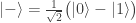 and, by the Born rule, Bob is equally likely to measure as .
Thus depending on Alice’s measurement, the vector in Hilbert space (equivalently one of Rudolph’s ‘misty states’, or the ‘wavefunction’ in the language of the EPR paper) describing Bob’s qubit may take two different values. Except for changing ‘position’ to -basis and ‘momentum’ to -basis, this is the same situation as on page 779 of the EPR paper, where the authors write
We see therefore that as a consequence of two different measurements performed upon the first system, the second system may be left in states with two different wavefunctions. On the other hand, since at the time of measurement the two systems no longer interact, no real change can take place in the second system in consequence of anything that may be done to the first system. This is, of course, merely a statement of what is meant by the absence of an interaction between the two systems. Thus, it is possible to assign two different wavefunctions … to the same reality (the second system after the interaction with the first).
The authors conclude that the wavefunction is, like the rocky state of the flipped coin above, an incomplete description of reality. Repeating Rudolph’s argument from page 104 quoted above, since two different rocky states correspond to the same real state, the rocky state cannot be a physical property of the coin. This is consistent with (but does not imply in its full strength) naive realism.
The expectation of the EPR authors, if I understand the history correctly, was that quantum mechanics would be subsumed by a larger theory — maybe with ‘hidden variables’ — whose states would, everyone could agree, be in bijection with physical reality. Even the term ‘hidden variable’ now seems pejorative, but this idea of a progression of understanding by a sequence of more and more refined theories is of course entirely consistent with the history of physics.
Note the quote makes it very clear that the EPR authors do not regard Alice’s act of measurement as an interaction with Bob’s qubit. This assumption should seem doubtful given the game discussed in Part 2, where we saw that the improvement in the winning chance from to depended on Alice and Bob being able to influence the correlation between their measurements of their shared Bell state by careful choice of bases, using only locally available information. Indeed Bell’s 1964 paper concludes that this improvement is inconsistent with a local hidden variable theory:
In a theory in which parameters are added to quantum mechanics to determine the results of individual measurements, without changing the statistical predictions, there must be a mechanism whereby the setting of one measuring device can influence the reading of another instrument, however remote. Moreover, the signal involved must propagate instantaneously, so that such a theory could not be Lorentz invariant.
This puts us back where we were at the end of Part 2, forced to accept the spooky ‘action at a distance’ effect of measuring. This non-locality was the central problem for Einstein with the theory: on the inability to measure Bob’s qubit in both the – and -bases he wrote `es ist mir wurst’ (literally, ‘it is a sausage to me’). I’m happy to agree: I think scientific realism can easily stretch to accommodate measurements whose precision is limited by the uncertainty principle, and even to ruling out as simply nonsensical the idea of measuring both the position and momentum of a particle at the same instant. (Like the – and -matrices, position and momentum are conjugate Hermitian operators.) More worrying perhaps, we are left with no better candidates for the ultimate elements of reality that Rudolph’s misty states. Rudolph admits the problems (page 81):
Such a mist would … have to have many physical properties that differ from any other kind of physical stuff we have ever encountered. It would be arbitrarily stretchable and move instantaneously when you whack it at one end, for example. The whole question of how to interpret the mist—as something physically real? as something which is just mathematics in our heads?—is one of the major schisms between physicists.
I would have liked to see it mentioned here that even if Alice’s measurement does, as experimentally verified, instantaneously affect Bob’s qubit, it appears to be impossible to use this effect to transmit information. To be fair, Rudolph does consider this point carefully, but only later in Part 3. This distinction is particularly relevant in the context of quantum teleportation, which I discuss next.
Quantum teleportation
Most accounts of quantum teleportation that I have seen begin with the circuit below.
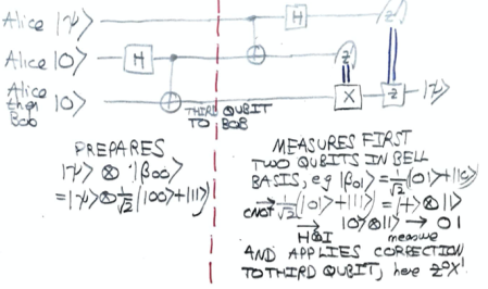
Alice begins in control of three unentangled qubits. The first is in the state  that she wants to teleport to Bob. After applying the Hadamard and CNOT gates, Alice sends the third qubit to Bob. She then applies another CNOT gate, a Hadamard gate and measures her two qubits in the -basis. (Why?, you might well ask.) She sends the two classical bits that are the results of her measurements to Bob by a classical channel, marked as double blue lines in the diagram. Finally Bob applies a correction by and gates and, as if by magic, obtains
  .
.
I think I would have got the idea rather more quickly if the circuit diagram had been accompanied by the explanations below:
- The circuit left of the red dashed line prepares the Bell state on the second and third qubits.
- The CNOT gate and Hadamard gate on the right of the red dashed line transform the Bell basis to the -basis. One example is shown above, another is
 which is sent by the CNOT gate to
 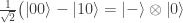 and then by the Hadamard gate to
  .
.
- By the identity

when Bob applies the corrections from the classical bits sent by Alice, he obtains . (Note there is no ambiguity in  because
  and
and  stabilise . This identity follows easily from the calculations on page 83 of Quantum computing: A gentle introduction by E. Rieffel and W. Polak.)
Since learning the rudiments of the ZX-calculus, I also find the graphical proof that the circuit behaves as claimed quite satisfying. Note in particular that the Bell state is simply the cup (shown horizontally) on the left of the dashed red-line.
The algebraic view of the ‘yank’ that simplifies the ZX-calculus diagram is the identity

See (36) and (37) in ZX-calculus for the working computer scientist by John van de Wetering for more on this.
It is not hard to convince oneself that Bob cannot learn anything by observing the state  unless he knows at least one of the classical bits and sent to him by Alice. For instance, if is known by all to be a -basis element
  then Bob needs . (And in this case Alice might as well have sent the bit to Bob directly.) Thus while we believe that Alice’s measurements instantaneously affect Bob’s qubit, Bob cannot learn any information until light from Alice can reach Bob. This can be made precise using density matrices: the density matrix for Bob’s qubit is the uniform linear combination of the rank 1 density matrices for the four post-measurement states of the third qubit in the quantum teleportation protocol, namely

Setting 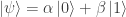 this becomes
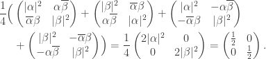
The right-hand side is the density matrix for the second qubit in the Bell state and is maximally uninformative: measurement in any orthonormal basis gives each basis vector with equal probability  .
.
In addition, quantum teleportation appears to be consistent with naive realism as defined above. Let and think of as a qubit that is with probability and is with probability . At the end of the protocol, this probability distribution is transferred from Alice’s qubit to Bob’s qubit. This is consistent with the idea that the qubit has a definite, but unknown state, to which this probability distribution refers.
In a classical analogue (which I learned from Prof. Ruediger Schack) this transfer of probability distributions can, and in fact must be interpreted entirely epistemically. The analogue of the Bell state is two coins in unknown but equal states: imagine Alice tapes coin 2 to coin 3, flips the composite coin, and then without looking at either coin, keeps coin 2, and gives coin 3 to Bob. The analogue of is a classical probability distribution on coin 1. In the protocol, Alice performs a parity measurement by performing another ‘tapped together flip’ on coins 1 and 2. She then looks at them both, and learns whether they are ‘same’ or ‘different’. She reports this to Bob, who then flips coin 3 if and only if Alice reports ‘different’.
Alice’s probability distribution now refers to coin 3: if Alice believed that coin 1 was heads with probability then she should now believe that Bob’s coin 3 is heads with probability . To show the epistemic character of this, imagine that coin 1 is prepared by a coin toss performed by Alice’s assistant Charlie, and that Alice does not look at the coin until after the parity measurement. If the coin is fair then Alice’s probability is , but Charlie’s probability is either or  . In each case, this probability refers to coin 3 at the end of the protocol. Even though can be any real number in the interval
 ![[0,1]](https://s0.wp.com/latex.php?latex=%5B0%2C1%5D&bg=ffffff&fg=333333&s=0&c=20201002) , it may now seem that no information is teleported, except the single classical bit from Alice’s ‘same’ or ‘different’.
, it may now seem that no information is teleported, except the single classical bit from Alice’s ‘same’ or ‘different’.
I think this makes it all a little more plausible that quantum states are incomplete descriptions of a deterministic theory, and that while this theory must include instantaneous ‘actions at a distance’ effects, it could be that such effects cannot be used to convey information, and so do not (from our human perspective) violate causality. And while we saw in the discussion of the PETE box in Part 1, that the realist point of view that qubits have a definite state — we just don’t know what it is until observation — requires hidden variables, the asymmetry between Alice and Charles seen above, and the epistemic interpretation of the ‘teleportation’, shows that the existence of such hidden information by no means impossible.
Discussion of Part 3
Rudolph begins this part by explaining that if misty states are real then the behaviour of the PETE box can be explained: for example the -basis state 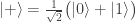 models a white ball output by a PETE box; if the next PETE box can ‘see’ this state then it can of course output a white ball in response. (That this happens by linear unitary evolution is nice for mathematicians, but potentially misleading: while linearity means we only have to state the effect of the Hadamard transformation on basis vectors, the behaviour of the PETE box, or rather the Stern–Gerlach magnetic fields, on superpositions is a property of the physical theory.) He also notes that this hypothesis does not require that misty states are a complete description of physical states.
The difficulty with this hypothesis is of course observation: why can PETE boxes observe -basis states without collapse, while human observation collapse everything we see into the -basis? We have seen that this act of observation requires instantaneous ‘action at a distance’ effects. Rudolph mentions attempts to make measurement compatible with unitary dynamics, writing (page 113)
But there are some models which work (at least for the ball type experiments we have considered; making them work for all experiments we can presently do is more tricky), and which soon will be experimentally ruled in or out.
Unhelpfully, no more details are given. He also mentions the ‘many worlds interpretation’ in which measurement splits the universe in two, in which the observer becomes a gigantic misty state representing a superposition of ‘observer saw black’ and ‘observer saw white’.
Next Rudolph considers the epistemic idea that misty states are ‘features of our knowledge, rather than real states of the world’ (page 115). He gives the argument from the EPR paper that since Alice’s measurement of her qubit in the entangled Bell pair can leave Bob’s qubit in two different misty states, and assuming that these measurements do not affect the physical properties of Bob’s qubit, two different misty states correspond to the same physical state, and so misty states cannot be physical properties. We saw above that the improvement from to in the winning probability for Bell’s game makes this assumption very doubtful; Rudolph makes the same point very clearly using his improved version of Bell’s game.
Rudolph goes on to illustrate, as usual in his toy model of black and white balls and PETE boxes, that measurements on an entangled Bell pair cannot be used to send information, by giving a special case of the calculation with density matrices above. The section concludes (page 126)
All this is mainly strange if you consider the mist to be real—if you follow Enstein and deny that the real state of Bob’s ball is changing at all then you should not expect them to be able to communicate in this manner.
But then how would you explain how the psychics won your gold?
The Bell game requires Alice and Bob to share the entangled Bell state; Rudolph’s improved version requires a slightly more complicated entanglement. Rudolph concludes with a demonstration that even separable quantum states show behaviour that is incompatible with naive realism as defined above. (He also paints Einstein as a naive realist, but on my understanding does not accurately reflect Einstein’s opinions by the end of his life.) Rudolph’s exposition features an entertaining dialogue between Einstein and Pooh Bear. I’ll present it rather more briefly here.
Suppose that Malcolm prepares one of the four states
 ,
, ,
, ,
, .
.
If, as in naive realism, we do not believe that misty states are themselves real, but instead think that is really either or (we just don’t know which until observation), then since any of the four states may give on observation, it is experimentally impossible to learn anything about which state was prepared. This however is false. We calculate that the output of the circuit shown below
is
 ,
, ,
, ,
, .
.
Now consider what happens when we measure the second qubit in the -basis.
- If it is measured as we measure the first qubit in the -basis; if the result of both measurements is
 then the initial state was not (1), if is
  then the initial state was not (4).
- If instead the second qubit is measured as then we apply a Hadamard gate to the first qubit, giving (1)
 , (2)
, (2)  , (3)
, (3)  , (4) , and then measure the first qubit in the -basis. Now from cases (2) and (3) we see that if the result of both measurements is the initial state was not (3), and if it is
  the initial state was not (2).
Therefore in all cases something can be deduced about the initial state.
Rudolph clearly explains that this result is inconsistent with naive realism but consistent with the view that physical states correspond to unique misty states. But, like Einstein, Rudolph finds the consequences of this, in particularly non-locality, hard to swallow. He concludes (page 139):
I personally live in cognitive dissonance: on a day-to-day basis I talk about the physical properties of the photons … as if they are as tangible as any of the physical properties of the human-scale objects in the room around me. They are not. I suspect I should treat the misty states as states of knowledge, but to be understood within a more general framework of theories of inference than our present theories find comfortable.
The idea that things may not be precisely as they present themselves to our senses has a long pedigree, going back as far as Plato and his shadows on the cave. Hume says it clearly in Section 118 in Enquiry concerning human understanding:
The table, which we see, seems to diminish, as we remove further from it. But the real table, which exists independently of us, suffers no alteration. If was therefore, nothing buts its image, which as present to the mind.
The tension here between things as they are (ontological properties) and things as they seem to us (epistemological properties) has of course been much debated by philosophers after Hume, most notably Kant with his noumena (or Ding an such) and phenomena. What we have seen in this post is that it may be impossible to maintain this separation: the EPR-paradox, Bell’s game, and Rudolph’s final demonstration all point to a theory in which the physical properties making up a real state includes a unique misty state. Moreover, neither the Stern–Gerlach experiment (with its random deflections), nor the EPR-paradox (with its spooky ‘action at a distance’), nor Rudolph’s final demonstration (quantum effects without initial entanglement) require the real state to be anything more than the misty state. But if this is true, it follows that our observed experience of phenomena cannot be disentangled with the ontological question: what is the nature of things as they really are?


 Posted by mwildon
  on a vector space
  and
and  . In particular the actions of
 ,
,  and
and  , a fact one would surely expect from the notation. The purpose of this post is to record a lemma about commuting group actions that arose in this context.
 and
and  . Then, for each
  , we have
 with
with  acting on the left on
  acting on the right, diagonally on each of the
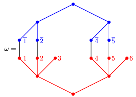
  factors, by permuting values. For instance, if
  and
and  then one joint orbit is
 ; a little thought shows that the stabiliser of
  is
is
 : even though we are working in
  , it is not the case that the stabiliser factors as
  .
. rather than the formally correct
  .
. .
. has the same
  where
where  is the subgroup of those
  fixing setwise the orbit
  . Moreover
  -modules
  .
. -modules
 as a
as a  -module in the second line and as a
  -module in the third line.
 is a normal subgroup of a permutation group
  then the orbits of
  . Then
  . This shows that
  and by symmetry equality holds.
 such that
  for some
  . The right-hand side is the set of cosets
  for some
  . These are equivalent conditions: take
  and use that the actions commute. Finally, identifying
  we see that
  . Since
  , as required.
 if and only if
  has a submodule isomorphic to
  and
and ![\dim V = [K : L]\dim U](https://s0.wp.com/latex.php?latex=%5Cdim+V+%3D+%5BK+%3A+L%5D%5Cdim+U&bg=ffffff&fg=333333&s=0&c=20201002) . In this case we take
. In this case we take  -module
  .
. for induction on the left, we can state the following corollary with left- and right-actions.
 is a left
 and
and  that respect the blocks
  ,
,  ,
,  ,
,  shown by the rooted trees in the graph below. The matching
  .
.
 and both
 . This is shown graphically below.
 . On the other hand, the permutation
  cannot be undone by a permutation in
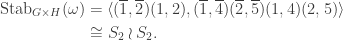
 .
. of
of  is a horizontal
  -border strip if there is a border-strip tableau
  of shape
  , to be
  where
where  is the sum of leg lengths in


 is replaced with an arbitrary partition, and
  with an arbitrary hook partition. I think the only reason he stopped at hook partitions was that this was the only case where there was a convenient combinatorial interpretation of a certain inner product (see the end of this subsection), because his argument easily generalizes to show that
 is any partition of
  (as before) and the second sum is over all
  . Since a one part partition has a unique
  then the only relevant
  is
is  . Hence a special case of Kochhar’s result, that generalizes the original result in only one direction, is
 . In the special case where
  , the plethystic Murnaghan–Nakayama rule states that
 is the product of
  and the size of a certain set of
  border-strip tableaux in which all the border strips have length
  and
and  and
and  . Below we will prove
 is a skew partition of
  , and the sums are over all
  and
and  are skew partitions.
 )
) are symmetric functions of degrees
  then
then
 on the ring of symmetric functions satisfies
  and the general fact
 .
. be the power sum symmetric function labelled by the partition
  . The expansion of an arbitrary homogeneous symmetric function
 is the size of the centralizer of an element
  of cycle type
  , where
  is the number of parts of size
  in
in 
 is the symmetric group character canonically labelled by the skew partition
 then, the coproduct relation implies that

 is an
is an  .
. in the power sum basis we get
 containing
 to define an
  elements. We saw in the preliminaries that, by the Murnaghan–Nakayama rule, if
  . Hence the right-hand side displayed above is
 for any symmetric functions
  (this is clear for

 relevant to
  be the set of semistandard tableaux of shape
  if and only if, in the rightmost column in which
  with
with  , this order becomes the colexicographic order on sets; similarly identifying semistandard tableaux of shape
  when
when  is shown below.
 is a
is a  denote the set of plethystic semistandard tableaux of shape
  are shown below.
 is in bijection with the set of partitions of
  box, by the map sending a partition
  entries equal to
  enumerates semistandard
  and writing, as is common,
  for
for  , we have
 enumerates plethystic semistandard tableau of shape
  for
for 
 denote the monomial symmetric function labelled by the partition
  since
since 
 . Moreover, by the duality
![\displaystyle \langle \mathrm{mon}_\lambda, h_\alpha \rangle = [\lambda = \alpha]](https://s0.wp.com/latex.php?latex=%5Cdisplaystyle+%5Clangle+%5Cmathrm%7Bmon%7D_%5Clambda%2C+h_%5Calpha+%5Crangle+%3D+%5B%5Clambda+%3D+%5Calpha%5D&bg=ffffff&fg=333333&s=0&c=20201002)
 , we have
 is the critical bridge we need from the combinatorics of plethystic semistandard tableaux to the decomposition of the plethysm
  . We require the following lemma.
 then
then  .
. , where
  is the permutation character of
  acting on
  . This leads to an alternative proof by orbit counting.
 , where
  is the number of partitions of
  then the multiplicities of
  in
in  and
and  agree: this verifies Foulkes’ Conjecture in the very special case of two row partitions. Moreover, specializing to two variables, it follows by conjugating partitions that
 is contained in
  which, by Young’s rule, has only constituents with at most
 if
if  if
if  and
and  , then the multiplicity of
  in
in  , independently of
  , let
, let ![\gamma_{[d]}](https://s0.wp.com/latex.php?latex=%5Cgamma_%7B%5Bd%5D%7D&bg=ffffff&fg=333333&s=0&c=20201002) denote the partition
denote the partition  . To avoid an unnecessary restriction in the theorem below we also define
 ![(1)_{[1]} = (1)](https://s0.wp.com/latex.php?latex=%281%29_%7B%5B1%5D%7D+%3D+%281%29&bg=ffffff&fg=333333&s=0&c=20201002) . For example, the lemma in the previous section that
. For example, the lemma in the previous section that ![s_{(r)_{[mn]}} = h_{(r)_{[mn]}} - h_{(r-1)_{[mn]}}](https://s0.wp.com/latex.php?latex=s_%7B%28r%29_%7B%5Bmn%5D%7D%7D+%3D+h_%7B%28r%29_%7B%5Bmn%5D%7D%7D+-+h_%7B%28r-1%29_%7B%5Bmn%5D%7D%7D&bg=ffffff&fg=333333&s=0&c=20201002) . We generalize this in the first lemma following the theorem below.
. We generalize this in the first lemma following the theorem below.![\langle s_n \circ s_m, s_{\gamma_{[mn]}} \rangle](https://s0.wp.com/latex.php?latex=%5Clangle+s_n+%5Ccirc+s_m%2C+s_%7B%5Cgamma_%7B%5Bmn%5D%7D%7D+%5Crangle&bg=ffffff&fg=333333&s=0&c=20201002) is independent of
is independent of  .
. and
and  . Let
. Let  . For each partition
  there exist unique coefficients
  for
for  such that
![s_{\gamma_{[d]}} = \sum_{\beta \in L} b_{\beta} h_{\beta_{[d]}}.](https://s0.wp.com/latex.php?latex=s_%7B%5Cgamma_%7B%5Bd%5D%7D%7D+%3D+%5Csum_%7B%5Cbeta+%5Cin+L%7D+b_%7B%5Cbeta%7D+h_%7B%5Cbeta_%7B%5Bd%5D%7D%7D.&bg=ffffff&fg=333333&s=0&c=20201002)
 and
and  unless
  .
.![h_{\beta_{[d]}} = \sum_{\gamma \in L} K_{\beta_{[d]}\gamma_{[d]}} s_{\gamma_{[d]}}, (\ddagger)](https://s0.wp.com/latex.php?latex=h_%7B%5Cbeta_%7B%5Bd%5D%7D%7D+%3D+%5Csum_%7B%5Cgamma+%5Cin+L%7D+K_%7B%5Cbeta_%7B%5Bd%5D%7D%5Cgamma_%7B%5Bd%5D%7D%7D+s_%7B%5Cgamma_%7B%5Bd%5D%7D%7D%2C+%28%5Cddagger%29&bg=ffffff&fg=333333&s=0&c=20201002)
 is the number of semistandard Young tableaux of shape
  unless
  , we are justified in summing only over elements of
  in
in  .
. be the set of semistandard tableaux of shape
 ![\beta_{[d]}](https://s0.wp.com/latex.php?latex=%5Cbeta_%7B%5Bd%5D%7D&bg=ffffff&fg=333333&s=0&c=20201002) and content
and content  , there are
  entries of
  , these
  . This leaves
  boxes in the top row to be occupied by entries
  , where the only restriction is that these entries are weakly increasing. Therefore there is a bijection between
  and content
 ![K_{\beta_{[d]}\gamma_{[d]}} = \widetilde{K}_{\beta\gamma},](https://s0.wp.com/latex.php?latex=K_%7B%5Cbeta_%7B%5Bd%5D%7D%5Cgamma_%7B%5Bd%5D%7D%7D+%3D+%5Cwidetilde%7BK%7D_%7B%5Cbeta%5Cgamma%7D%2C&bg=ffffff&fg=333333&s=0&c=20201002)
 , we have
  , and since
  unless
  . The lemma now follows by inverting the unitriangular matrix
  .
.  , the size of the set
 ![\mathrm{PSSYT}\bigl((n), (m)\bigr)_{\gamma_{[mn]}}](https://s0.wp.com/latex.php?latex=%5Cmathrm%7BPSSYT%7D%5Cbigl%28%28n%29%2C+%28m%29%5Cbigr%29_%7B%5Cgamma_%7B%5Bmn%5D%7D%7D&bg=ffffff&fg=333333&s=0&c=20201002) is independent of
is independent of  then any
  and weight
 ![\gamma_{[mn]}](https://s0.wp.com/latex.php?latex=%5Cgamma_%7B%5Bmn%5D%7D&bg=ffffff&fg=333333&s=0&c=20201002) has
has  then the first
 ![\mathrm{PSSYT}\bigl((n),(m))_{\gamma_{[mn]}}](https://s0.wp.com/latex.php?latex=%5Cmathrm%7BPSSYT%7D%5Cbigl%28%28n%29%2C%28m%29%29_%7B%5Cgamma_%7B%5Bmn%5D%7D%7D&bg=ffffff&fg=333333&s=0&c=20201002) and
and ![\mathrm{PSSYT}\bigl((n-1),(m-1)\bigr)_{\gamma_{[(m-1)(n-1)]}}](https://s0.wp.com/latex.php?latex=%5Cmathrm%7BPSSYT%7D%5Cbigl%28%28n-1%29%2C%28m-1%29%5Cbigr%29_%7B%5Cgamma_%7B%5B%28m-1%29%28n-1%29%5D%7D%7D&bg=ffffff&fg=333333&s=0&c=20201002) .
.  or
or  , the multiplicities
 ![\langle s_n \circ s_m, h_{\beta_{[mn]}}\rangle](https://s0.wp.com/latex.php?latex=%5Clangle+s_n+%5Ccirc+s_m%2C+h_%7B%5Cbeta_%7B%5Bmn%5D%7D%7D%5Crangle&bg=ffffff&fg=333333&s=0&c=20201002) are independent of
are independent of  be the set of integer sequences
  such that
  for all
  and
and  . Given
  and a partition
  is also a partition, we define
  to be the maximum number of single box moves, always from longer rows to shorter rows, that take the Young diagram of
  .
. and
and  , the maximum number of moves is
  , then one box from row
  , and finally one box from row
  to row
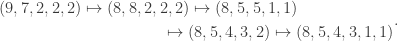
 ; since one box must be moved directly from row
  , and an upper bound for
  of an expression for
  . For instance, again with
 . In general, we have
 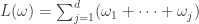 , or, equivalently,
 be such that
  . The plethysm coefficient
  is constant for
  and the stable value is
  .
. for a partition
  and the claim gives the stability bound in the Foulkes case
  be the natural representation of the general linear group
  . In conventional Schur—Weyl duality, one uses the bimodule
  , acted on diagonally by
  on the right to pass between polynomial representations of
 must be replaced with some larger algebra. For the orthogonal group one obtains the
  , one obtains the
  be the collection of set partitions of
  . The symmetric group
  be the corresponding permutation module defined over
  and let
  be the corresponding permutation character. For instance the permutation character appearing in Foulkes’ Conjecture of
  . In this case, each set partition in
  has stabiliser
  ; in general a stabiliser is a direct product of wreath products acting on disjoint subsets.
 denote the set of partitions of
 ![\langle s_{(n)} \circ s_{(m)}, s_{\gamma_{[mn]}}\rangle](https://s0.wp.com/latex.php?latex=%5Clangle+s_%7B%28n%29%7D+%5Ccirc+s_%7B%28m%29%7D%2C+s_%7B%5Cgamma_%7B%5Bmn%5D%7D%7D%5Crangle&bg=ffffff&fg=333333&s=0&c=20201002) is equal to
is equal to  .
.![S^{\gamma_{[mn]}}](https://s0.wp.com/latex.php?latex=S%5E%7B%5Cgamma_%7B%5Bmn%5D%7D%7D&bg=ffffff&fg=333333&s=0&c=20201002) in the permutation module
in the permutation module  . They then apply Schur—Weyl duality to move to the partition algebra, defined with parameter
  . In this setting, the Specht module
  for the partition algebra canonically labelled by
  from
from  corresponding to
 ![[V^{(m^n)} : \Delta_r(\gamma)]_{S_{mn}} = \sum_{\beta \in \mathrm{Par}_{\ge 2}(r)} [P^\beta : S^\gamma]_{S_r}.](https://s0.wp.com/latex.php?latex=%5BV%5E%7B%28m%5En%29%7D+%3A+%5CDelta_r%28%5Cgamma%29%5D_%7BS_%7Bmn%7D%7D+%3D+%5Csum_%7B%5Cbeta+%5Cin+%5Cmathrm%7BPar%7D_%7B%5Cge+2%7D%28r%29%7D+%5BP%5E%5Cbeta+%3A+S%5E%5Cgamma%5D_%7BS_r%7D.&bg=ffffff&fg=333333&s=0&c=20201002)
 agree.
 . Here it is very helpful that the natural representation
  , making it not too hard to describe all the embeddings of the representation
  into the tensor product
  case, the analogue of the set
  of set partitions of
  into disjoint sets of sizes
  , now with one subset marked. Let
  be the corresponding permutation character. Let
  be the set of partitions of
  . The multiplicity
 ![\langle s_{(n-1,1)} \circ s_{(m)}, s_{\gamma_{[mn]}}\rangle](https://s0.wp.com/latex.php?latex=%5Clangle+s_%7B%28n-1%2C1%29%7D+%5Ccirc+s_%7B%28m%29%7D%2C+s_%7B%5Cgamma_%7B%5Bmn%5D%7D%7D%5Crangle&bg=ffffff&fg=333333&s=0&c=20201002) is stable for
is stable for  and
and  .
. lying in
  are
are  ,
,  and
and  with corresponding permutation modules induced from
  ,
,  , and
, and  . (This example is atypical in that the subgroups are all Young subgroups; in general they are products of wreath products.) The sum of the permutation charaters is
  from which one can read off the stable multiplicities of
 ![s_{\gamma_{[mn]}}](https://s0.wp.com/latex.php?latex=s_%7B%5Cgamma_%7B%5Bmn%5D%7D%7D&bg=ffffff&fg=333333&s=0&c=20201002) in
in ![s_{(4)_{[mn]}}](https://s0.wp.com/latex.php?latex=s_%7B%284%29_%7B%5Bmn%5D%7D%7D&bg=ffffff&fg=333333&s=0&c=20201002) has stable multiplicity
has stable multiplicity  be the set of pairs
  where
where  having exactly
  into parts all of size
  and
and  , where
  is the multiplicity of
  as a part of
  is a Young subgroup of
  and
and  is a subgroup of
  , where
  , and
, and  has its conventional meaning.
 of
of  . Then inflate to the product of wreath products
 be a partition of
 ![\langle s_{\kappa_{[n]}} \circ s_{(m)}, s_{\gamma_{[mn]}}\rangle](https://s0.wp.com/latex.php?latex=%5Clangle+s_%7B%5Ckappa_%7B%5Bn%5D%7D%7D+%5Ccirc+s_%7B%28m%29%7D%2C+s_%7B%5Cgamma_%7B%5Bmn%5D%7D%7D%5Crangle&bg=ffffff&fg=333333&s=0&c=20201002) is stable for
is stable for  and
and 
 is defined by
 .
. in the left-hand side of the inner product in the theorem is
 . Therefore the case
  of the theorem recovers the original result of Bowman and Paget.
 has
has  for a unique
  in the sense of the previous section. In this case
 from the previous section. Therefore again the theorem specializes as expected.
 when
when  . It will be convenient shorthand to write
  for the Young permutation character induced from the trivial representation of the Young subgroup
  . The decomposition of each
  has five marked set partitions.
 : here

 : here
  and so we compute
 and
and  , respectively. More simply, these are
  and
and  . Hence
 . (This is a bit of a coincidence I think, but convenient for calculation.) Therefore
  and
and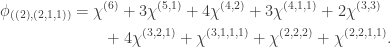
 . A similar argument to the previous case shows that
 ,
,
 : here
  and so we compute
  . Inflating and inducing we find that
 , we have
 : here
  and so the restriction map does nothing. We then inflate to get
  . The induction of this character to
  is
is
 .) The displayed character above is
  .
. and
and  ,
,![\begin{aligned} & s_{(n-3,2,1)} \circ s_{(m)} = \\ &\quad \cdots + 4s_{(6)_{[mn]}} \!+\! 11s_{(5,1)_{[mn]}} \!+\! 11s_{(4,2)_{[mn]}} \!+\! 7s_{(4,1,1)_{[mn]}} \\ &\qquad \!+\! 4s_{(3,3)_{[mn]}} \!+\! 8s_{(3,2,1)_{[mn]}} \!+\! s_{(3,1,1,1)_{[mn]}} \!+\! s_{(2,2,2)_{[mn]}}\\ &\qquad \!+\! s_{(2,2,1,1)_{[mn]}} \!+\! \cdots \end{aligned}](https://s0.wp.com/latex.php?latex=%5Cbegin%7Baligned%7D+%26+s_%7B%28n-3%2C2%2C1%29%7D+%5Ccirc+s_%7B%28m%29%7D+%3D+%5C%5C+%26%5Cquad+%5Ccdots+%2B+4s_%7B%286%29_%7B%5Bmn%5D%7D%7D+%5C%21%2B%5C%21+11s_%7B%285%2C1%29_%7B%5Bmn%5D%7D%7D+%5C%21%2B%5C%21+11s_%7B%284%2C2%29_%7B%5Bmn%5D%7D%7D+%5C%21%2B%5C%21+7s_%7B%284%2C1%2C1%29_%7B%5Bmn%5D%7D%7D+%5C%5C+%26%5Cqquad+%5C%21%2B%5C%21+4s_%7B%283%2C3%29_%7B%5Bmn%5D%7D%7D++%5C%21%2B%5C%21+8s_%7B%283%2C2%2C1%29_%7B%5Bmn%5D%7D%7D+%5C%21%2B%5C%21+s_%7B%283%2C1%2C1%2C1%29_%7B%5Bmn%5D%7D%7D+%5C%21%2B%5C%21+s_%7B%282%2C2%2C2%29_%7B%5Bmn%5D%7D%7D%5C%5C+%26%5Cqquad++%5C%21%2B%5C%21+s_%7B%282%2C2%2C1%2C1%29_%7B%5Bmn%5D%7D%7D+%5C%21%2B%5C%21+%5Ccdots+%5Cend%7Baligned%7D&bg=ffffff&fg=333333&s=0&c=20201002)
 where
where  . This decomposition can be verified in about 30 seconds using Magma.
 we have
![\langle s_{\kappa_{[n]}} \circ s_{(m)}, s_{\gamma_{[mn]}} \rangle = \langle \psi^\kappa_r, \chi^\gamma \rangle.](https://s0.wp.com/latex.php?latex=%5Clangle+s_%7B%5Ckappa_%7B%5Bn%5D%7D%7D+%5Ccirc+s_%7B%28m%29%7D%2C+s_%7B%5Cgamma_%7B%5Bmn%5D%7D%7D+%5Crangle+%3D+%5Clangle+%5Cpsi%5E%5Ckappa_r%2C+%5Cchi%5E%5Cgamma+%5Crangle.&bg=ffffff&fg=333333&s=0&c=20201002)
 we have, for each partition
 into parts of sizes
  ,
,  . Hence
 . Denote this character by
  . By the restated version of the theorem,
![\langle s_{(k)_{[n]}} \circ s_{(m)}, s_\gamma \rangle = \sum_{(\alpha,\beta)\in\mathrm{MPar}_k(r)} \langle \rho^{(\alpha,\beta)}, \chi^\gamma\rangle.](https://s0.wp.com/latex.php?latex=%5Clangle+s_%7B%28k%29_%7B%5Bn%5D%7D%7D+%5Ccirc+s_%7B%28m%29%7D%2C+s_%5Cgamma+%5Crangle+%3D+%5Csum_%7B%28%5Calpha%2C%5Cbeta%29%5Cin%5Cmathrm%7BMPar%7D_k%28r%29%7D+%5Clangle+%5Crho%5E%7B%28%5Calpha%2C%5Cbeta%29%7D%2C+%5Cchi%5E%5Cgamma%5Crangle.&bg=ffffff&fg=333333&s=0&c=20201002)
 we find that
![\langle s_{(k)_{[n]}} \circ s_{(m)}, 1_{S_r}\rangle = |\mathrm{MPar}_k(r)|,](https://s0.wp.com/latex.php?latex=%5Clangle+s_%7B%28k%29_%7B%5Bn%5D%7D%7D+%5Ccirc+s_%7B%28m%29%7D%2C+1_%7BS_r%7D%5Crangle+%3D+%7C%5Cmathrm%7BMPar%7D_k%28r%29%7C%2C&bg=ffffff&fg=333333&s=0&c=20201002)
 and
and  which we have seen is
 and partitions of
  , as required.
 . It is known that a plethysm
 ![s_\nu[1-X]](https://s0.wp.com/latex.php?latex=s_%5Cnu%5B1-X%5D&bg=ffffff&fg=333333&s=0&c=20201002) , was given by Langley and Remmel: see Theorem 3.1 in their paper
, was given by Langley and Remmel: see Theorem 3.1 in their paper ![s_\lambda[s_\mu]](https://s0.wp.com/latex.php?latex=s_%5Clambda%5Bs_%5Cmu%5D&bg=ffffff&fg=333333&s=0&c=20201002) at hook and near-hook shapes
at hook and near-hook shapes .
. . To get started take
  . Since
  is a Littlewood–Richardson product of the transitive permutation characters
  for
for  , and a Littlewood–Richardson product is a hook only when every term in the product is a hook, the stable hook constituents
  are precisely the hook partitions in
 is the number of semistandard Young tableaux of shape
  . This is the Kostka number
 , and so the longest leg length of a stable hook grows as
  . (We emphasise that all this follows from the original result of Bowman and Paget.)
 , using the generalization proved above, then the
  contributes further parts
  to the content above, and so the stable hook multiplicity is
 with multiplicity
  with multiplicity
  are
are  ,
,  ,
,  ,
,  , of which the final three each defines a unique semistandard Young tableau counted by the Kostka number above; the contents are
  ,
,  and
and  respectively.
 to compute. We can build a list of the first
  . The reason is that under lazy evaluation, only the existence of each entry of the list has to be established; each
  .
.
 questions are necessary and sufficient, where
  is the number of
  . Since black and white balls are equally balanced in the remaining components and
  , the balls in the component of size
  are in the majority. (We will see later that this generalises to multiple colours.) Moreover, since the sum of component sizes expresses
  questions; the final question graph is a tree. When
  possible sets of black balls (for each partition
  one may colour the larger set black), and so we must learn
  be the colour of ball
  . This is
  where
where 
 is odd.
 . We immediately note that if
  , and so we can determine a ball’s colour in just one evaluation, making (1) trivial. For (2), the first
  evaluations are necessary and sufficient. For (3) the obvious strategy uses
  when
when  , to find the colour of every ball using
  . (Equivalently,
  .) Begin by evaluating
  for
for  . Suppose that the results are
 , exactly one of

 balls
balls  such that
  . Since
  we are again in the happy position of being able to learn a ball’s colour with a single evaluation. This gives a strategy for game (1) using
  evaluations. For game (2) we use
  evaluations
 ; this is possible since
  .
. .
. by noting that
  . If distinct arguments are required then one can use
  such that
  ; then

 , we must require distinct arguments to avoid the reduction to Problem 1. With this condition, observe that if
 , and since swapping
  affected the majority, we must also have
  ; now
; now  for any
  at disjoint triples
  until both values
 and
and  , one can find
  with
with  and there are just two white balls. We identify
  with
with  and cover the
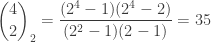
 . Since there are
  distinct
  evaluations (plus those to find
  then there are
  lines, and so
  questions are needed is lost.
 is odd. If we evaluate
  of the
  balls) and get
  black balls and at most
  questions, and for game (3) using
  questions.
 and
and  is now
  . Components in the question graph are now labelled by
  up to cyclic permutation. For example, when
  contains
  balls of colour
  and no balls of colour
  , for some
  . A comparison of a ball in the component
  with one in the component
  unites the components as
 such balls) or correctly declare that all colours occur equally often, in a third, the aim is to find a ball of plurality colour (knowing that black balls are in plurality).
 bits of information are learned in each evaluation, we might expect fewer questions to be necessary than in the usual majority game. On the other hand, the greater number of colours gives the adversary more options. What are optimal strategies for the cyclic
  , the value is
  , the value is
  questions, claiming in a terminal position has three components. One optimal line of questioning follows a Binary Knight Hunt to reach the position


 above, a move connecting the components
  results in either
  ,
,  or
or  and in all cases a majority ball is now known. But without the restriction, the next position may be
  and no majority ball can be identified. Another subtle point is that the next position cannot be
  , since this has no colour in the majority.
 and
and  may be united as
 , the value of
  and the balanced components have sizes
  . Let black be the majority colour. If balls in the uniform component of size
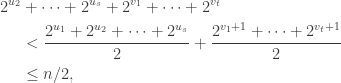
 and
and  comparisons are necessary and sufficient to find a black ball.
 ,
,  may give
  . The main result is impressively sharp: if
  and
and  questions are needed to identify a ball whose colour is in a plurality.
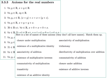
 ,
,  ,
,  is correct in this gap? `Whatever you think, half the people disagree with you … do you want to change your mind?’.
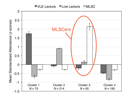
 return, their mean has variance
  , so mathematically is a safer investment. (This is the basis of the infamous Collatoralized Debt Obligation, peddled enthusiastically by investment banks such as Goldman Sachs who rewarded their clients by then betting against the asset they had just purchased.) As the 2008 Financial Crisis showed, the independence assumption is utter garbage. Yet another worrying example comes from the use of machine learning in sentencing algorithms: the algorithm
  . An
. An ![[7,4,3]](https://s0.wp.com/latex.php?latex=%5B7%2C4%2C3%5D&bg=ffffff&fg=333333&s=0&c=20201002) –Hamming code
–Hamming code  to be the linear code of length
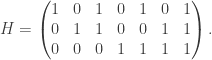

 . Since the disjoint Hamming balls of radius
  binary words of length
  , these balls partition
  . Therefore
  containing
  .
. permutes the
  . Let
. Let  be the position permutation of the columns of
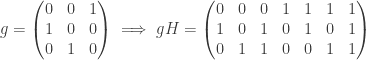
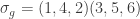 . (Since I am hyper-paranoid about such things, I will verify that
  is a homomorphism by comparing
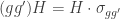 , where
  denotes the column permutation action.) Now writing
  for the permutation matrix of
 ![P(\sigma)_{ij} = [i\sigma = j]](https://s0.wp.com/latex.php?latex=P%28%5Csigma%29_%7Bij%7D+%3D+%5Bi%5Csigma+%3D+j%5D&bg=ffffff&fg=333333&s=0&c=20201002) ), we have
), we have
 . If
. If  then the left-hand side is
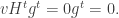
 , and indeed the image of the homomorphism
  and correspondingly,
  is a codeword in
 .
.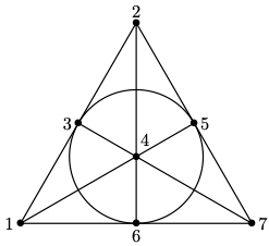
 as
as  where
where  . The binary quadratic residue code of length
  whose generator polynomial has as its roots the powers of
 of
of  . Thinking of
  of
of ![\mathbb{F}_2[x]/\langle x^7+1 \rangle](https://s0.wp.com/latex.php?latex=%5Cmathbb%7BF%7D_2%5Bx%5D%2F%5Clangle+x%5E7%2B1+%5Crangle&bg=ffffff&fg=333333&s=0&c=20201002) , we have
, we have  if and only if
  . From this it is easy to see that
  .) The same argument holds for the cyclic code
  whose generator polynomial is
  is defined using the
  .
. . Since
  is an automorphism of
  . To obtain the rest, we need the following two claim.
 then the position permutation
  preserves
  . This deals with the case
  , and
, and  is obtained by squaring.
  then the position permutation
  sends
sends  and
and  sends
sends  is a root of
  .
.  and
and  . Setting
  we have
  . Since
  , and
, and  and
and  , we have
  . Hence
  ; since
  . Similarly
  . Hence
  and we have the required automorphism.
 is replaced with the Riemannian metric
  , putting time on the same footing as space. As one would expect from this author, the consequences are worked out in great detail, and are integral to the plot. This comes at some predictable expense to characterisation and versimilitude: still I’ve found the first two books sufficiently interesting that I can (almost) ignore that much of the exposition consists of the characters giving each other physics tutorials, conducting experiments (which remarkably always work, even if the results often come as a surprise) or listening to each other give lectures and seminars. That said, the physics is leavened by some set-piece ethical dilemmas, and there is also a well-developed biological theme, concentrated on the unique (but not completely implausible) morphology of the Orthogonal race.
 that light travels in this interval, space-time has the Lorentz metric
  . For example, a photon may move from
  to
to  in one unit of time, and, corresponding to the fact that no time passes for the photon, the Lorentz distance between these space-time points is zero.
 , where
  to its world line called its
  and in the Orthogonal universe
  . A stationary observer measures the particle’s velocity as the
  , as illustrated in the diagram below (click for a larger pdf).
 , where
  is the
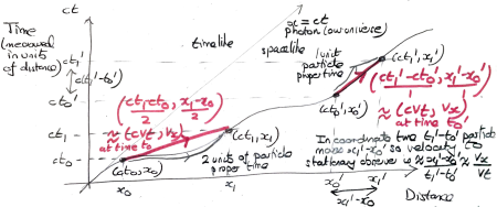
 is dimensionless (while the constant
  in the diagram above, it is multiplied by
  -plane has clocks every metre, connected by rigid rods, which record the time of passing of every particle. The particle is at position
  (which conveniently enough happens to have a clock) at time
  , and at position
  (similarly conveniently placed) at time
  . The stationary observer can therefore collect the measurements from the clocks (simply by travelling to each one), and approximate the particle’s velocity as
  and so
  . Everyday objects in our universe, such as cars, trains and coronavirus, move at a negligible fraction of the speed of light, so
  is typically huge compared to
  , and corresponding the velocity measured by the observer is a tiny fraction of the speed of light.
 for the
  for the square of its
 . By symmetry invariance, the Lorentzian norm squared of the tangent vector is
  , and the Euclidean norm squared is
  (using the assumption that
  ). Now since
  has units distance/time, and we care only about the direction of the tangent vector, not its magnitude, it is most convenient (and usual in physics, although I’ve never seen it clearly explained why) to require, as in axiom (3), that the Lorentzian length is
  , and so
  , where
  is the usual dimensionless Lorentz factor. In the Orthogonal universe
  ; this is again dimensionless because the
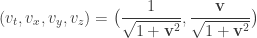
 , so fast moving particles are lighter according to a stationary observer.
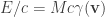 in our universe, and
  in the Orthogonal universe. Substituting in the
  has Lorentzian length
  , and in the Orthogonal universe,
 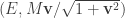 has Euclidean length
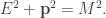
 and
and  , where
 ![\Gamma \in [0, \pi/2]](https://s0.wp.com/latex.php?latex=%5CGamma+%5Cin+%5B0%2C+%5Cpi%2F2%5D&bg=ffffff&fg=333333&s=0&c=20201002) . The analogue for our universe, using the identity
. The analogue for our universe, using the identity  , is
, is 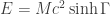 and
and  . We show both by the triangles below, noting that only the Orthogonal triangle is a genuine geometric representation, rather than a helpful aide-memoire.
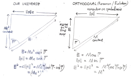
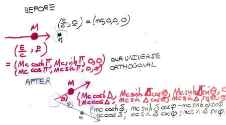
 -space (of which the diagram above shows only the
  -plane), so all
 and observe that for our universe

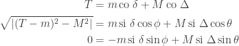
 are
are  in our universe and
  in the Orthogonal universe. The expression
  is positive in our universe and negative for the Orthogonal universe; it has the three constants
  ,
,  . The graph below show the post-collision velocity
 .
.
 , so is lower for faster moving particles.
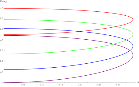
 , we obtain
 . Multiplying the top equation by
  and the bottom equation by
  and subtracting, we obtain
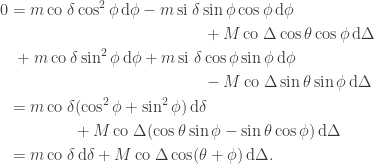
 and
and  , so the same sign appears both times, we get
 and
and  , we see that the coefficients must be in the same ratio: that is
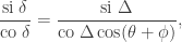
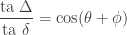
 is
is  in our universe and
  in the Orthogonal universe.
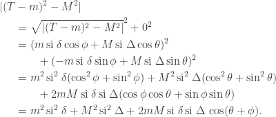
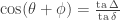 . Substituting and using


 , that
 for our universe and
  for the Orthogonal universe. Using these two relations to eliminate
  and
and  and recalling that
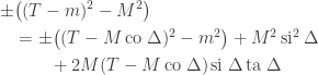
 appears. After multiplying through by
  we can simplify the right-hand side as follows
 on each side and rearranging, we get the final equation

 we immediately get
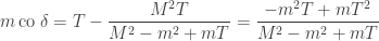

 and
and  into the equation from the tangent space equation
  we obtain
 of the left-hand fraction becomes
  if
if  , and so vanishes if
  . (Of course only the specialization
  is
is  . Hence we have
 simplifies to

 we get
 we get by a rearrangement and squaring the following quadratic equation in
 . (This is one of several places where we can see that there is a maximum deflection angle if and only if
  .) Since
  , and, as claimed some time ago, the sine of the maximum deflection angle is simply the ratio of the masses.
 above now implies that
 is the total energy (up to the factor
  in our universe), is that it depends on which universe we are working in only by a change from the hyperbolic function
  (our universe) to the trigonometric function
  (Orthogonal universe). Moreover, the maximum deflection angle
  Pascal’s Triangle matrix defined by
  , where, as in the
  be the shifted Pascal’s Triangle matrix defined by
  . Let
. Let ![J(n)_{xy} = [x+y=n-1]](https://s0.wp.com/latex.php?latex=J%28n%29_%7Bxy%7D+%3D+%5Bx%2By%3Dn-1%5D&bg=ffffff&fg=333333&s=0&c=20201002) be the involution reversing the order of rows (or columns) of a matrix, and let
be the involution reversing the order of rows (or columns) of a matrix, and let
 ,
,  and
and  for readability in proofs.
 , and any
  , the matrix
  is an involution.
 , the matrix is not the identity. Since
  we have
![\begin{aligned} \bigl( D^\pm B_a D^\pm B_a \bigr)_{xz} &= (-1)^x \sum_y (-1)^y \binom{x+a}{y+a} \binom{y+a}{z+a} \\ &= (-1)^x \sum_y \binom{x+a}{z+a}\binom{x-z}{y-z}(-1)^y \\ &= (-1)^{x+z} \binom{x+a}{z+a} \sum_r \binom{x-z}{r}(-1)^r \\ &= (-1)^{x+z} \binom{x+a}{z+a} [x=z] (-1)^{x+z} \\ &= [x=z] \end{aligned}](https://s0.wp.com/latex.php?latex=%5Cbegin%7Baligned%7D+%5Cbigl%28+D%5E%5Cpm+B_a+D%5E%5Cpm+B_a+%5Cbigr%29_%7Bxz%7D+%26%3D+%28-1%29%5Ex+%5Csum_y+%28-1%29%5Ey+%5Cbinom%7Bx%2Ba%7D%7By%2Ba%7D+%5Cbinom%7By%2Ba%7D%7Bz%2Ba%7D+%5C%5C+%26%3D+%28-1%29%5Ex+%5Csum_y+%5Cbinom%7Bx%2Ba%7D%7Bz%2Ba%7D%5Cbinom%7Bx-z%7D%7By-z%7D%28-1%29%5Ey+%5C%5C+%26%3D+%28-1%29%5E%7Bx%2Bz%7D+%5Cbinom%7Bx%2Ba%7D%7Bz%2Ba%7D+%5Csum_r+%5Cbinom%7Bx-z%7D%7Br%7D%28-1%29%5Er+%5C%5C+%26%3D+%28-1%29%5E%7Bx%2Bz%7D+%5Cbinom%7Bx%2Ba%7D%7Bz%2Ba%7D+%5Bx%3Dz%5D+%28-1%29%5E%7Bx%2Bz%7D+%5C%5C+%26%3D+%5Bx%3Dz%5D+%5Cend%7Baligned%7D&bg=ffffff&fg=333333&s=0&c=20201002)

 and
and  .
. . Hence
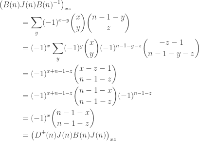
 has order
  we have
![\begin{aligned} \bigl( D^\pm & J B D^\pm J B D^\pm J B \bigr)_{xw} \\ &= (-1)^x \sum_y \sum_z (-1)^{y+z} \binom{n-1-x}{y}\binom{n-1-y}{z} \\ & \hspace*{3in} \binom{n-1-z}{w} \\ &= (-1)^{x+n-1} \sum_z \Bigl( \sum_y \binom{n-1-x}{y} \binom{-z-1}{n-1-y-z} \Bigr) \\& \hspace*{3in} \binom{n-1-z}{w} \\ &= (-1)^{x+n-1} \sum_z \binom{n-2-x-z}{n-1-z}\binom{n-1-z}{w} \\ &= (-1)^{x} \sum_z (-1)^{z}\binom{x}{n-1-z}\binom{n-1-z}{w} \\ &= (-1)^{x+n-1} \sum_r (-1)^r \binom{x}{r} \binom{r}{w} \\&= (-1)^{x+n-1} (-1)^x [x=w] = (-1)^{n-1}. \end{aligned}](https://s0.wp.com/latex.php?latex=%5Cbegin%7Baligned%7D+%5Cbigl%28+D%5E%5Cpm+%26+J+B+D%5E%5Cpm+J+B+D%5E%5Cpm+J+B+%5Cbigr%29_%7Bxw%7D+%5C%5C+%26%3D+%28-1%29%5Ex+%5Csum_y+%5Csum_z+%28-1%29%5E%7By%2Bz%7D+%5Cbinom%7Bn-1-x%7D%7By%7D%5Cbinom%7Bn-1-y%7D%7Bz%7D+%5C%5C+%26+%5Chspace%2A%7B3in%7D+%5Cbinom%7Bn-1-z%7D%7Bw%7D+%5C%5C+%26%3D+%28-1%29%5E%7Bx%2Bn-1%7D+%5Csum_z+%5CBigl%28+%5Csum_y+%5Cbinom%7Bn-1-x%7D%7By%7D+%5Cbinom%7B-z-1%7D%7Bn-1-y-z%7D+%5CBigr%29+%5C%5C%26+%5Chspace%2A%7B3in%7D+%5Cbinom%7Bn-1-z%7D%7Bw%7D+%5C%5C+%26%3D+%28-1%29%5E%7Bx%2Bn-1%7D+%5Csum_z+%5Cbinom%7Bn-2-x-z%7D%7Bn-1-z%7D%5Cbinom%7Bn-1-z%7D%7Bw%7D+%5C%5C+%26%3D+%28-1%29%5E%7Bx%7D+%5Csum_z+%28-1%29%5E%7Bz%7D%5Cbinom%7Bx%7D%7Bn-1-z%7D%5Cbinom%7Bn-1-z%7D%7Bw%7D+%5C%5C+%26%3D+%28-1%29%5E%7Bx%2Bn-1%7D+%5Csum_r+%28-1%29%5Er+%5Cbinom%7Bx%7D%7Br%7D+%5Cbinom%7Br%7D%7Bw%7D+%5C%5C%26%3D+%28-1%29%5E%7Bx%2Bn-1%7D+%28-1%29%5Ex+%5Bx%3Dw%5D+%3D+%28-1%29%5E%7Bn-1%7D.+%5Cend%7Baligned%7D&bg=ffffff&fg=333333&s=0&c=20201002)
 denote the half-turn rotation of an
  . By Claim 3,
 and so to
  . Hence this matrix has order
  has order
  has order
  . If
. If  has order